Intuitive explanation of bayes theorem – Part 2/2
In my previous article about Bayes theorem I attempted to explain in a simple way the main ideas behind the formula. Today, let's take it to another level! I'll show you a way that allows you to update your prior beliefs given new information. Some people call this way to use the Bayes Theorem the diachronic Bayes because it evolves through time with new information ! Indeed, you update your believes as you collect more evidence.
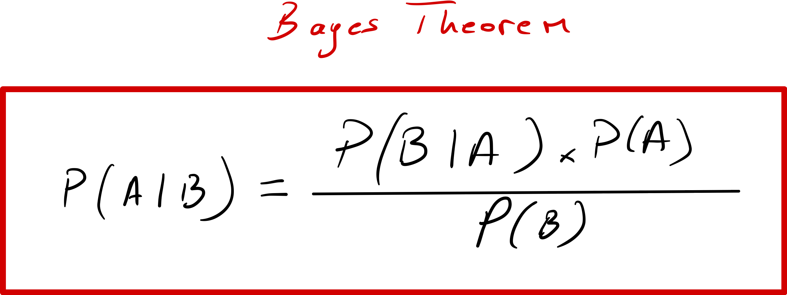
Recall the Bayes Theorem:
Now let's just chage a bit the notation and Introduce the notions of "hypothesis" and "Data"
Let H be hypothesis and D be the Data, the formula becomes:
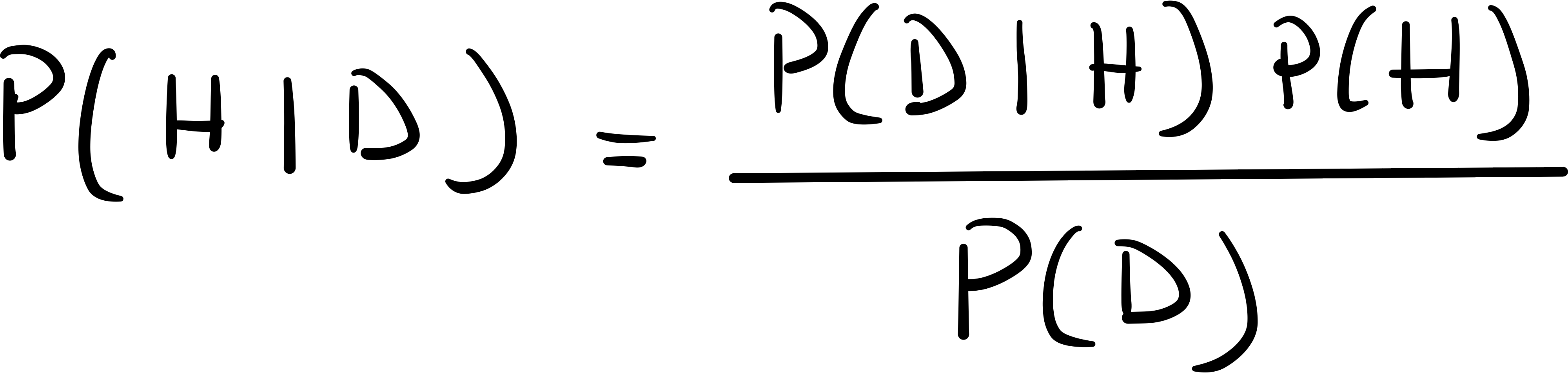
Note that it's not the "final form" of the formula, generally we expand the denominator so it can be calculated. Recall that in my previous blog post we used the law of total probability to expand it.
The idea is to break P(D) into smaller pieces, I've prepared a little drawing to make it clearer (feel free to read my previous article if it's still not crystal clear).
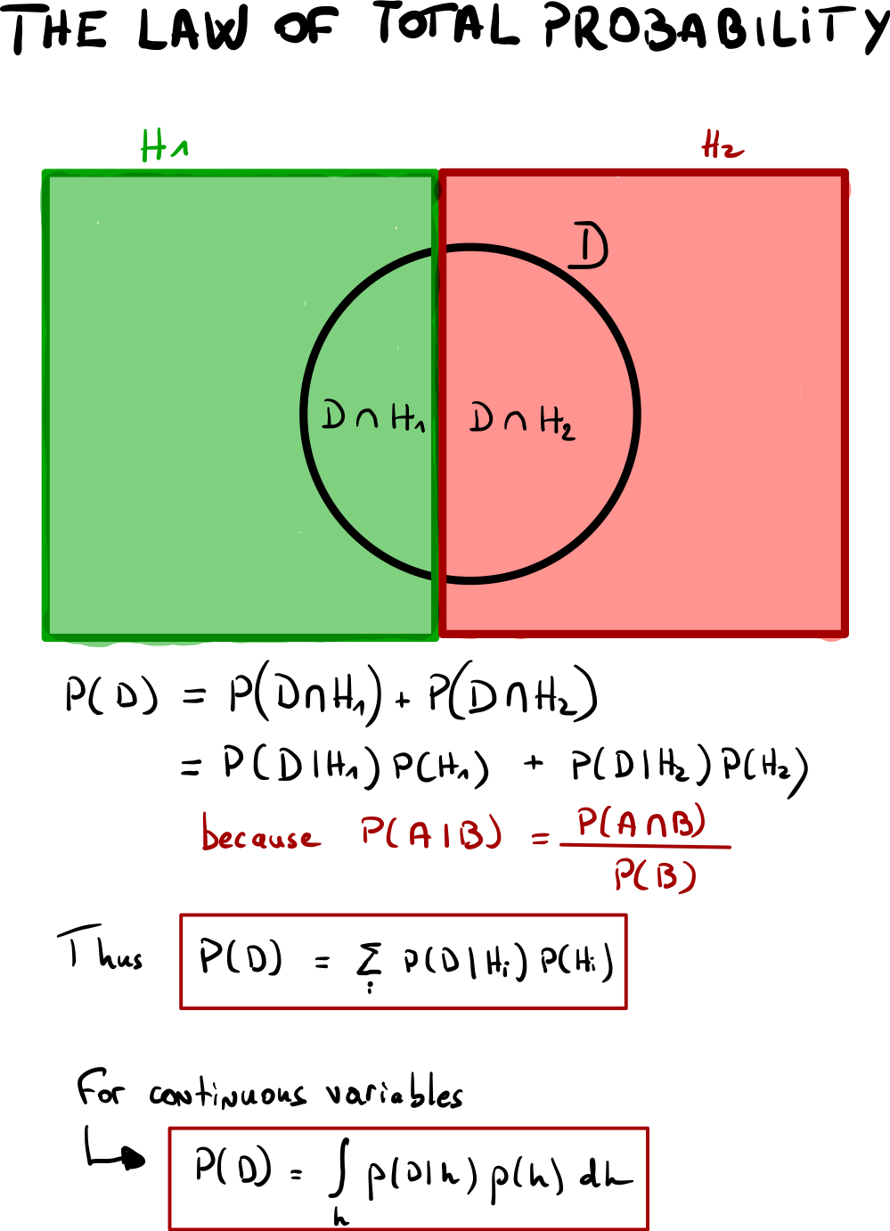
The smaller pieces must form a partition of D which meach that they are mutually exclusives (no overlap between the pieces) and colletively exhaustive (the sum of the pieces equals D).
If you find these notations somewhat enigmatic for now, don't worry we will dive into an example shortly, hopefully it will be clearer.
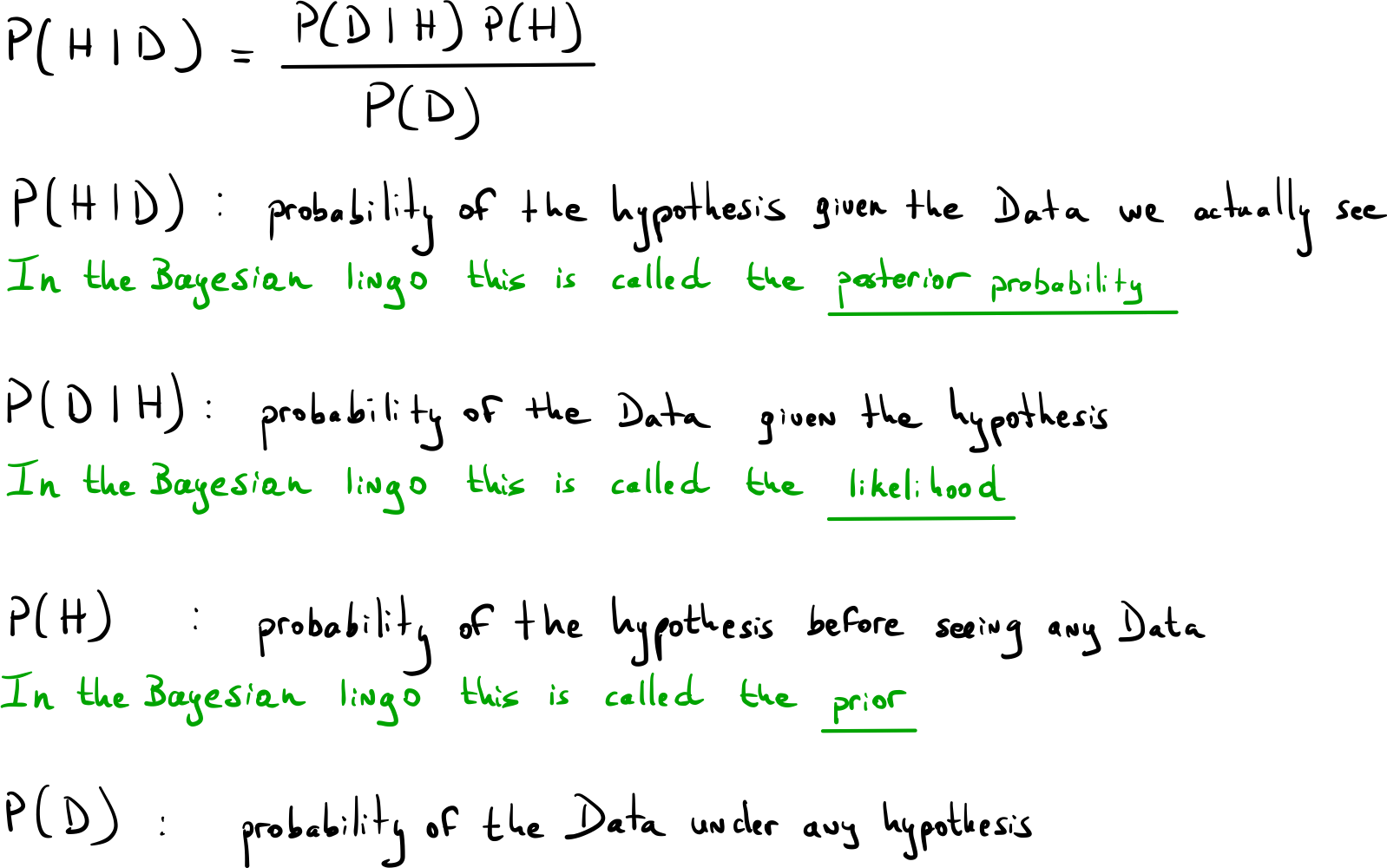
Before that, I'd like to comment a bit each quantity of the Bayes formula.
P(H | D)
This is called the posterior probability because it's the result you get after applying the bayes theorem. It gives you the probability of the hypothesis given the Data. This quantity is equal to the Likelihood times Prior divided by the probability of the Data.
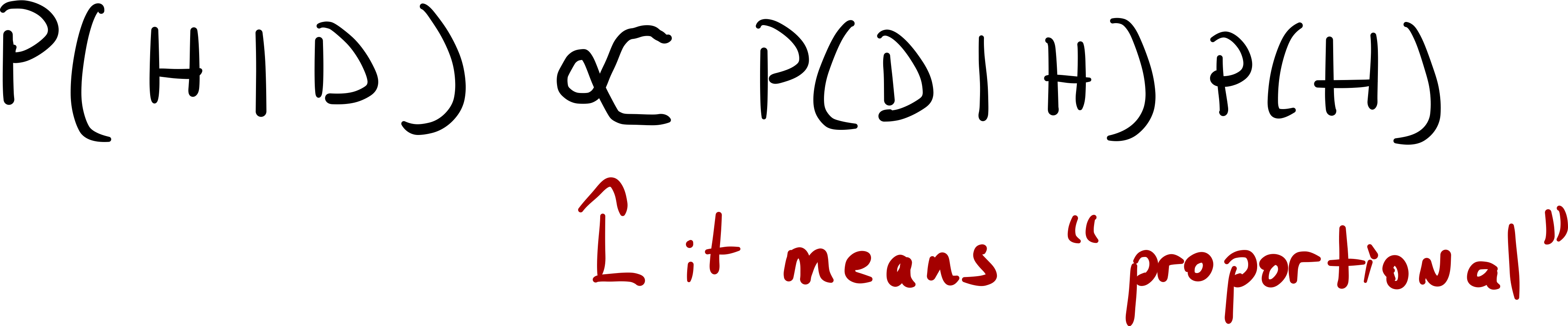
Generally we don't mention P(D) at all, instead we just say that P(H | D) is proportional to the Likelihood x Prior.
P(D)
This is the probability of the Data, This quantity might sound somewhat vague. As said before, we generally don't mention it at all because most of the time we don't actually need it (at least at first). We can notice that the denominator (which is P(D) ) in the "expanded" version of the Bayes theorem is in reality the same expression as the numerator.
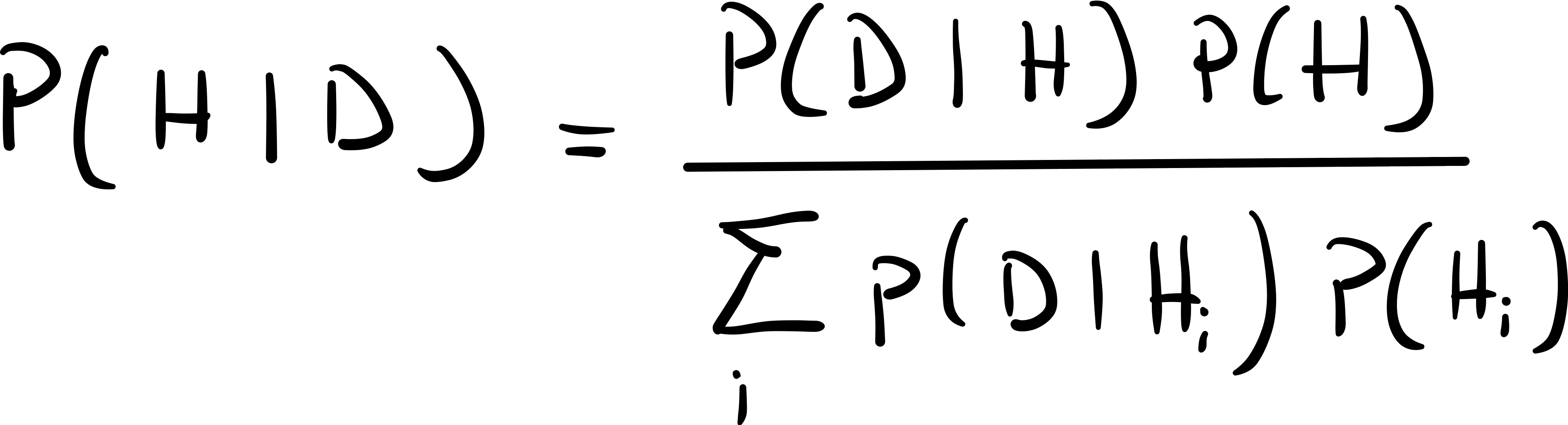
The only difference is that It sums over all the possible hypothesis. So in fact when you calculated all the P(D | H_i)P(H_i) you can just sum them together and the result would be equal to P(D) (Again this is just the law of total probability). In fact, this quantity can be seen as a normalizing constant that makes all the probabilities add up to 1. In other words we don't really have to worry about P(D) and explicitly calculate it at first, you'll be able to find it a the last step of your calculation, you'll see in the example :) .
Note that this quantity can be very hard to calculate in some cases, especially for continuous variables that involve tricky distributions. That won't be the case in our example.
P(H)
This is called the prior because it reflects your prior belief about the hypothesis. Generally this probability comes from the general knowledge or a study or sometimes it's only a subjective value which can be seen as prejudices. This is the reason why sometimes bayesian statistics are criticized and controversial.
You are at a party and Bob would like too introduce you to some of his friends. Some of them have a bad reputation, they are konwn to be nasty. During the party you meet 3 groups of friends. Now the party is over, it's time to go home you decide to order an uber but you can't find your mobile phone. A kind person in the party comes to you and tells you that she saw someone dressed in black stealing your phone but she can't figure out exactly who this guy was.
Suppose that for each group of friends the people stayed together all party long which means they didn't mix up with other groups.
In the first group there were 3 people dressed in Black and 5 with other colors.
In the second group there were 6 people dressed in Black and 5 with other colors
In the third group there were 5 people dressed in Black and 4 with other colors
Group 1 --> B: 3 | O: 5
Group 2 --> B: 6 | O: 5
Group 3 --> B: 5 | O: 4
Also, you have no clue which group has done this, which means that each group has a priori the same probability of guilt
Which group has a posteriori the highest probability of containing the thief ?
Recall the formula:

We want to calculate the probability of the hypothesis given the Data
Here the hypothesis are:
- H1: Group 1 is guilty
- H2: Group 2 is guilty
- H3: Group 3 is guilty
Let's calculate The probability associated with each hypothesis given the data so we can find the most probable scenario.
We have 2 quantities to really care about that is the likelihood P(D | H) and the prior P(H).
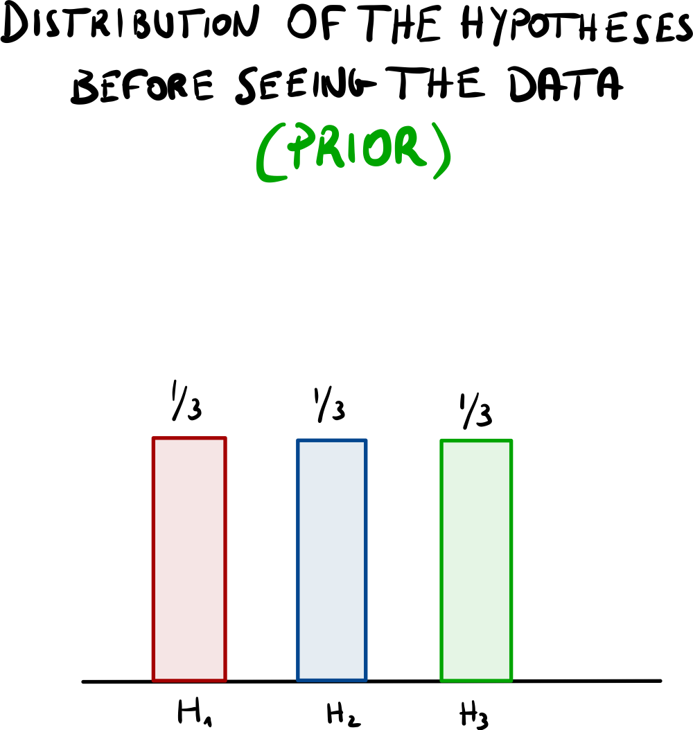
as each group has a priori the same probability of beeing guilty, the prior is distributed like so:
P(H = H1) = P(H = H2) = P(H = H3) = 1/3
(In the statistics lingo we also say that the variables are drawn from a uniform distribution.)
Now the likelihoods !
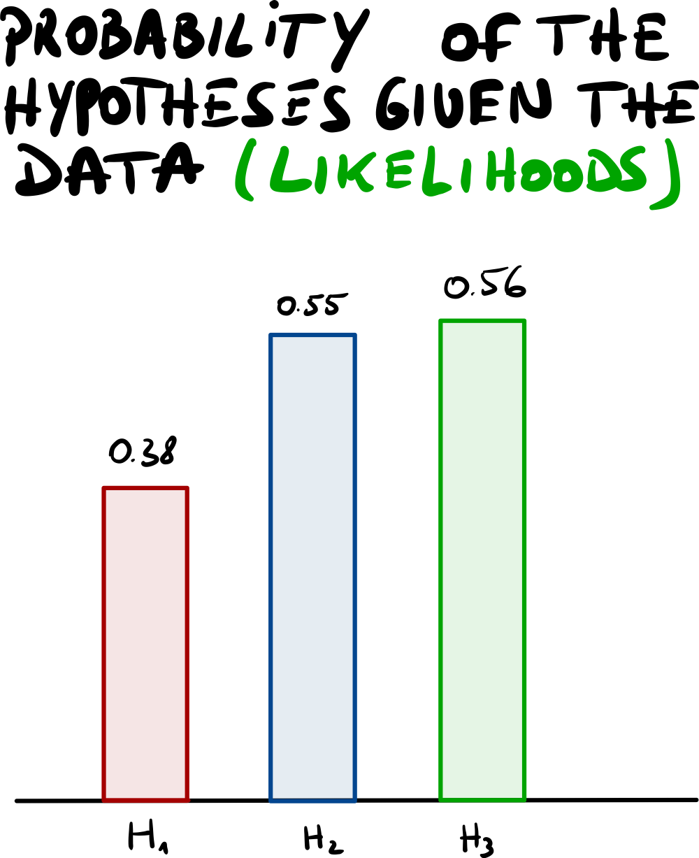
The likelihood is P(D | H).
The idea here is to use the fact that the thief is dressed in black to evaluate how likely a group is to be guilty.
- P(D = Black | H = Group 1) = 3/(3+5) = 0.38
- P(D = Black | H = Group 2) = 6/(6+5) = 0.55
- P(D = Black | H = Group 3) = 5(5+4) = 0.56
Now the work is almost done, we now have to multiply each Prior with its associated Likelihood.
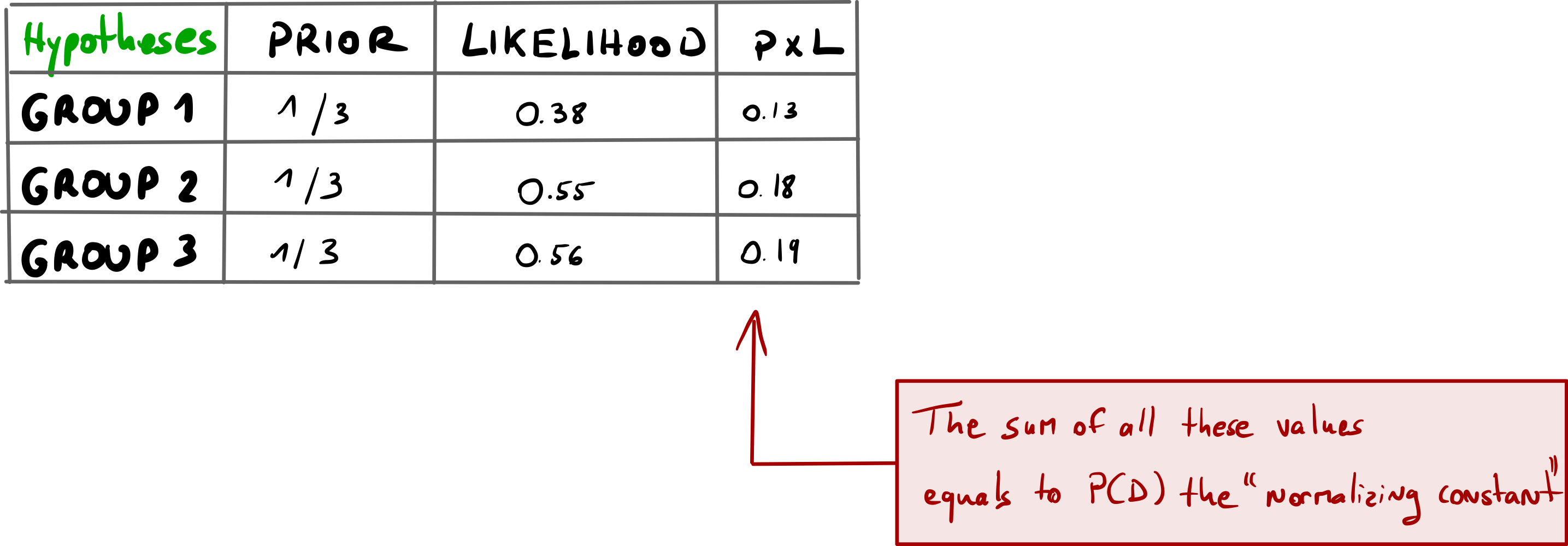
As you can see in the column PxL (Prior times Likelihood) the values don't add up to one. If we want to address this problem we simply have to divide each value by the sum of this column. In fact the sum of all theses values equals to P(D), what we have named "the normalizing constant". This gives us the Posterior.
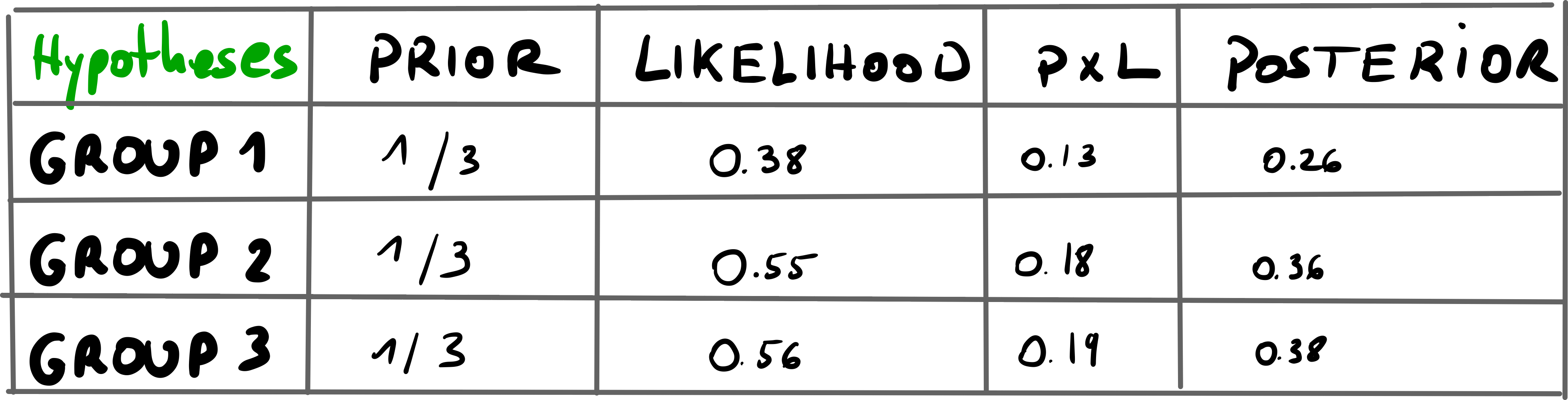
It turns out that group 2 and 3 have very close values
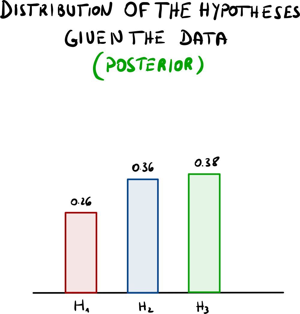
That data didn't help really...
But the nice thing about Diachronic Bayes is that you can save theses posterior probabilities somewhere and wait for new events. When you collect new data your prior distribution or belief won't be anymore 1/3, 1/3, 1/3 but it will be 0.26, 0.36, 0.38 as you gained new information with the data you gathered, in other words, you updated your believes.
Suppose now a friend of yours has experienced the same drama the day after you (yeah those people party every day :D ).
After the party your friend comes to you and you have a talk. He somehow managed to have more accurate likelihoods, that is:
- Group 1 Likelihood: 0.2
- Group 2 Likelihood: 0.25
- Group 3 Likelihood: 0.55
You decide to combine his information with yours. To be able to do that you take as a prior the posterior of your previous analysis and you associate it with the likelihoods of your friend.
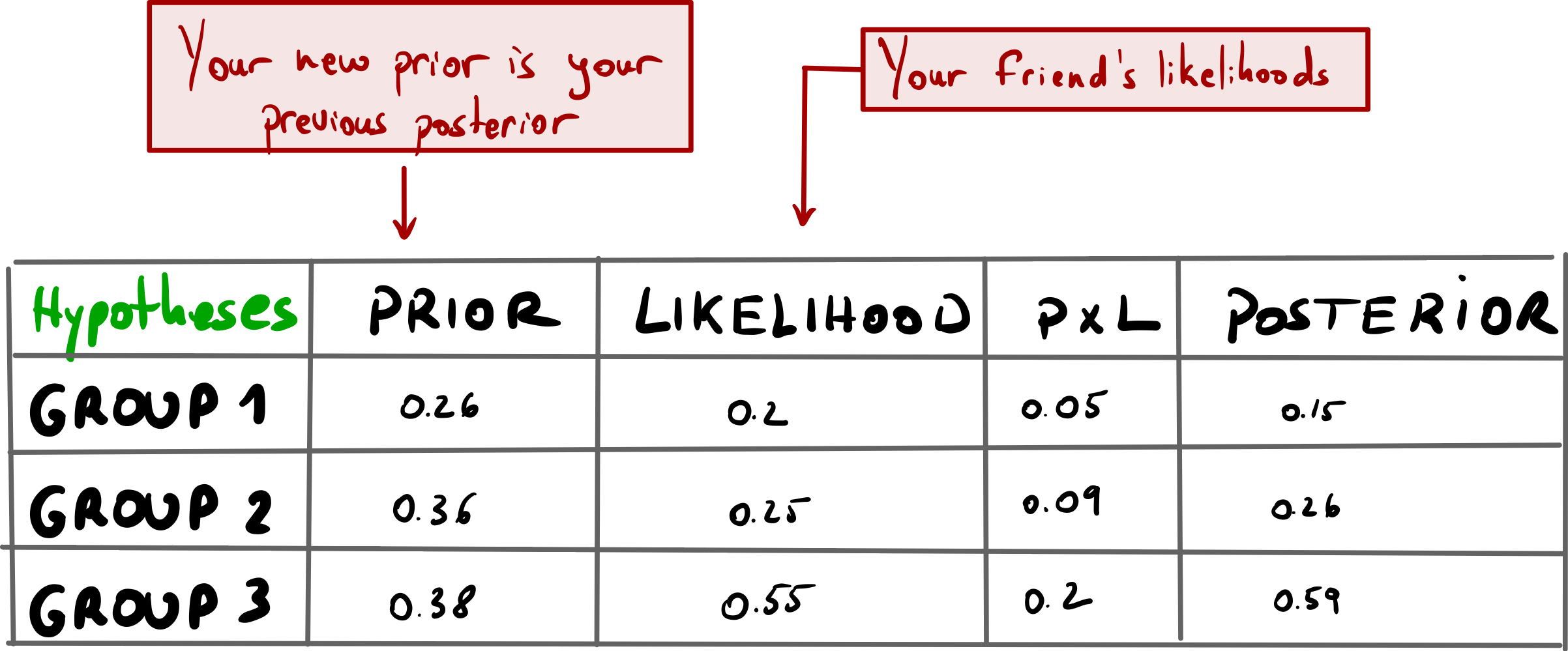
Let's draw the posterior distribution
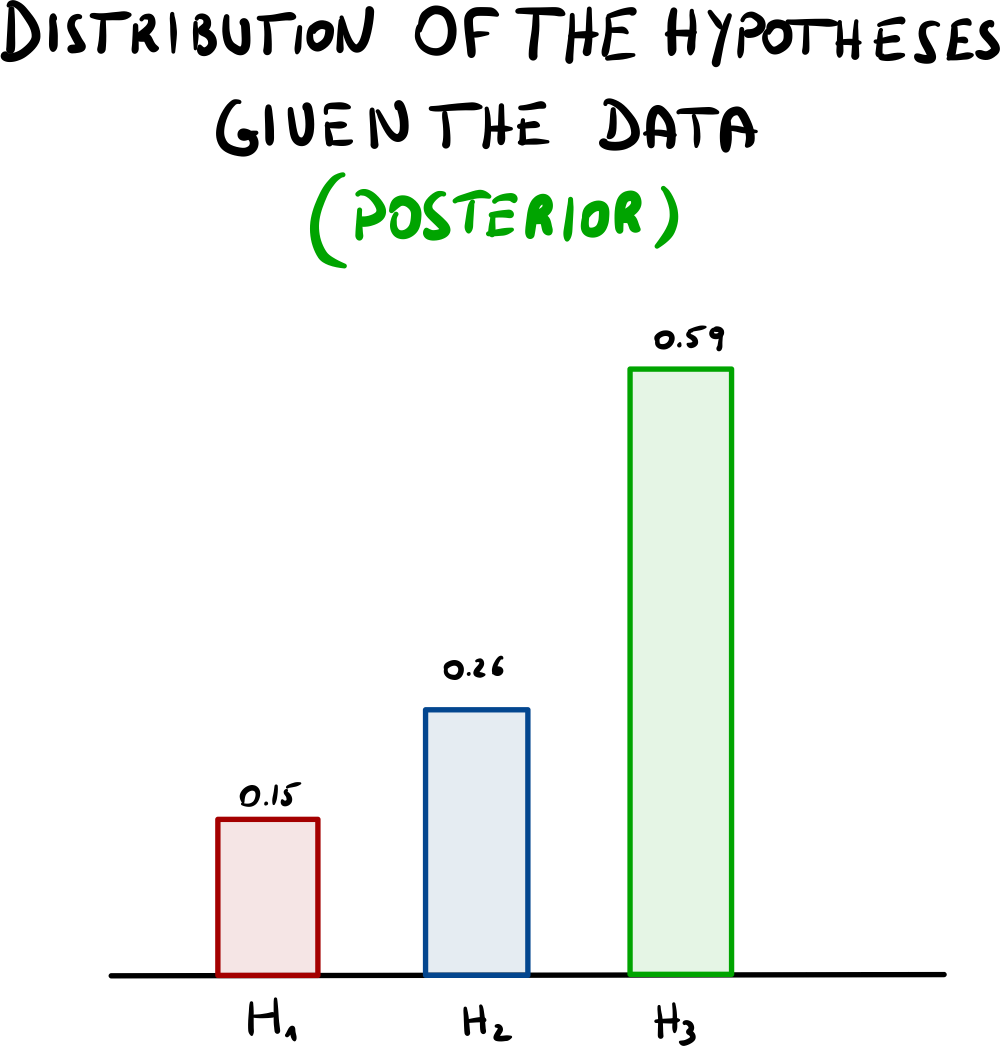
Okay... now that you gathered all the information you could get, the posterior distribution highly suggests that you should have a little talk with these nasty bad boys of the group 3 :D
Hopefully you now have a better understanding of how you can use Bayes Theorem in a diachronic way. This is the end of the article but there is still so much to talk about regarding Bayesian statistics. In particular Bayesian inference (how to predict new data), Bayesian networks (graphical models that represent probabilistic relationships between variables), Markov Chains Monte Carlo aka MCMC (allow for parameter estimation such as means, variances..., and exploration of tricky posterior distribution) but also the Naive Bayes Classifier (A machine learning model that uses Bayes Theorem).