What is Entropy ? — Intuitive explanation with code.
You may be familiar with variance, it is a useful measure when looking for how spread the data is. When I say spread, I'm referring to the dispersion of data around the sample's mean. Indeed, when the data is very spread it is often considered that it contains a lot of information. I say often because sometimes the data can be spread but it is not information, only noise. The concept of information is very important in Statistics and thus in Data Science. Entropy is one of those concepts that sounds magical at first and that is easily misunderstood and poorly taught. I'll try to keep this article as simple as possible, without using anything from information theory.
Consider those two examples:
A = [0, 0, 0, 0, 0]
B = [0, 1, 1, 2, 2]
In the list A there’s barely any information because the value is always the same, you won’t learn anything from there. In contrast, the list B contains several different values, which means you’ll probably learn something from it if those values are relevant. This concept might ring you a bell.
The concept of Entropy or Shannon Entropy has some similarities with variance. It is also a way to quantify the amount of information in the data. However, it is somewhat different than variance in the sense that it actually doesn’t care about the values themselves. Entropy is only interested in their probabilities. Let's stick with this idea of using probabilities to describe a system. Notice that in list A the probability associated with 0 is 100% but at the same time we said that there's no information. In this regard, we can say that the more uncertainty there is, the more information there is.
Let's put words on the previous lists and let say you want to choose a country for your summer holidays.
You want to choose the country so that you maximize the probability that the wether is sunny. The following lists contain the forecasts for the 5 coming days.
A = [Sunny, Sunny, Sunny, Sunny, Sunny]
B = [Sunny, Cloudy, Cloudy, Rainy, Rainy]
Now it becomes clear that you'll choose country A as country B has an uncertain weather (a high entropy)
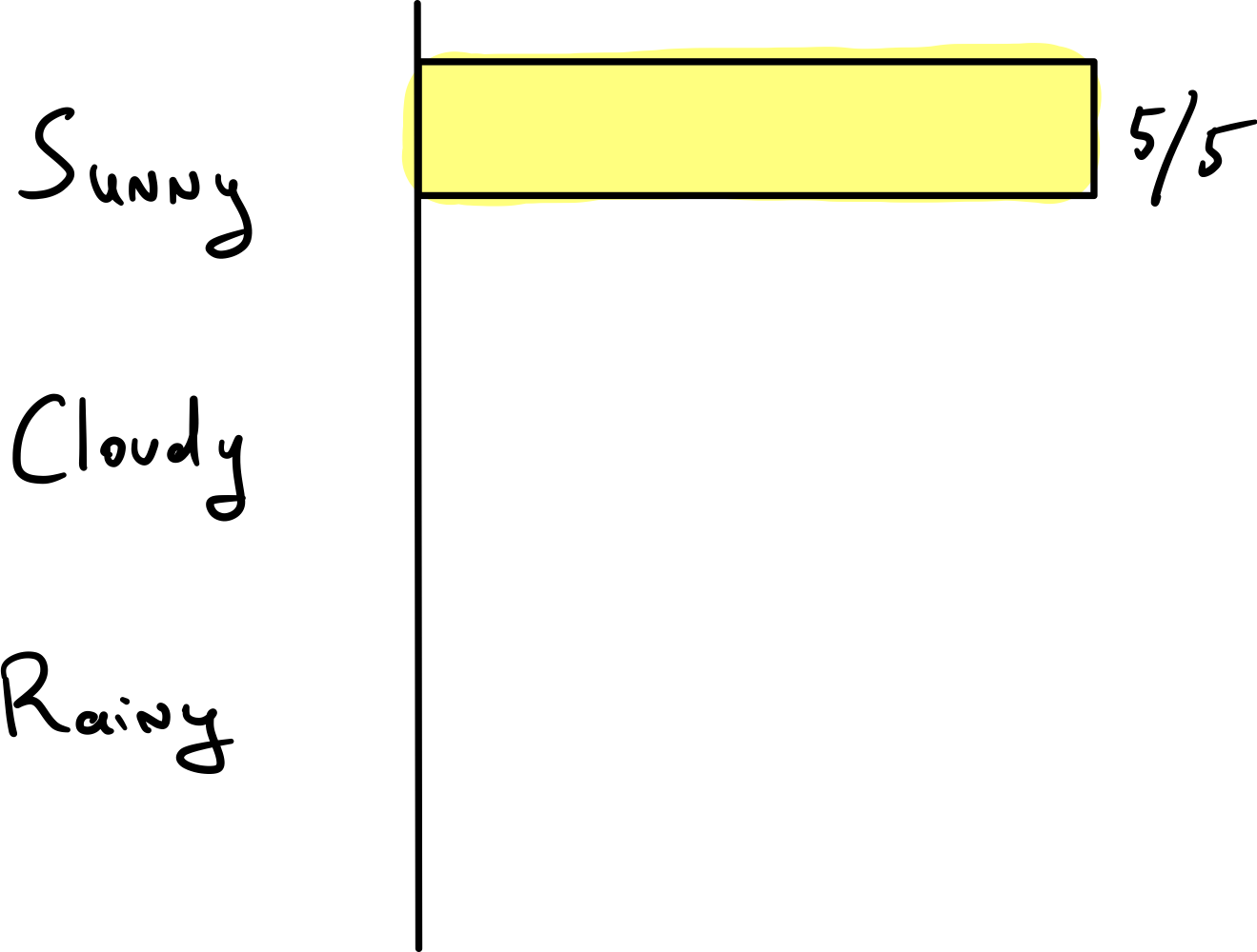
In this case, it's not very informative, thus it has low entropy.
In the second case, there is more variety (more information or higher entropy), the probabilities are spread across sunny, cloudy and rainy. With variety comes a way more complete information.
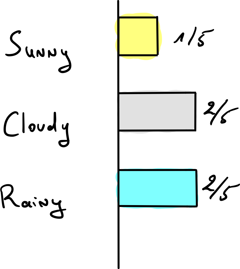
To put it in a nutshell, entropy is a way of quantifying uncertainty. This is probably the most intuitive way to see it. Uncertainty is inversely proportional to probability, that is to say, the more uncertain an outcome is, the least probable it is. As you might have guessed, the uncertainty is maximum when the distribution is uniform (all the probabilities are the same), basically it's a stalemate, it's chaos, you can't take any decision based on the probabilities... which is exactly the scenario where we said that information is maximum. Maximizing information is equivalent to maximizing uncertainty.
Intuition behind the formula
That's pretty much it, entropy is used to describe a probability distribution.
Now, I don't want to give you the formula yet, instead I would like to try to re-build it from scratch.
Imagine that you are given a bunch of different distributions and you have to find the one that has the least information/uncertainty. That is to say that the dream scenario would be to have one bar with 100% and 0% probability for all the others. The worst scenario would be to have all the probabilities equally distributed (note that what we do here is basically what's done in decision trees where we try to minimize uncertainty or impurity).
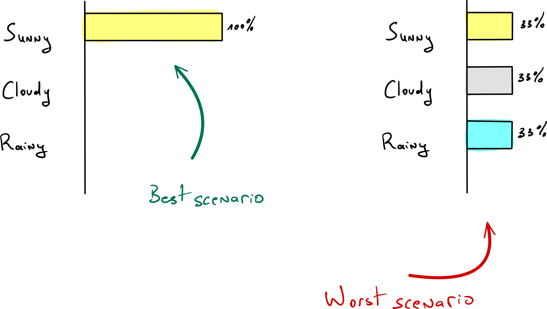
Now, with which formula/metric would you come up with to characterize theses states ?
The first thing I would try in this situation is to multiply all the probabilities together. The reasoning behind it is, as all the probabilities should add up to 1, one would expect that if a probability is very high, the others would be very low, thus all the tiny probabilities will make the whole product shrink to something near zero.
In contrast if the probabilities are all equally distributed, it prevents from having a very tiny probability that will make our product close to zero.
for instance:
A = [98%, 1%, 1%]--> 0.98 * 0.01 * 0.01 = 0.000098
B = [33%, 33%, 33%]--> 0.33 * 0.33 * 0.33 = 0.037
Note that I didn't want to take the scénario [100%, 0%, 0%] as it's obvious that any zero in the list would lead to a product of 0.
It looks like it's working ! B has the highest information/uncertainty. However it's quite annoying to deal with very small numbers (look at A). Multiplying many numbers smaller than 1 leads to very tiny results. A cool way to address this is to use the logarithm function because the product becomes a sum:
log(a*b) = log(a) + log(b)
Also, log is a monotonically increasing function, thus it doesn't change the relations of order.
A --> log(0.98 * 0.01 * 0.01) = log(0.98) + log(0.01) + log(0.01) = - 9.23
B --> log(0.33 * 0.33 * 0.33) = log(0.33) + log(0.33) + log(0.33) = -3.29
B remains the one that has the highest uncertainty and the numbers are not tiny !
But guess what, there's another issue. Indeed log(x) tends to -infinity when x approaches 0.
A trick to address this is to multiply log(p) by p because x*log(x) tends towards 0 when x approaches 0.
A --> 0.98*log(0.98) + 0.01*log(0.01) + 0.01*log(0.01) = - 0.11
B --> 0.33*log(0.33) + 0.33*log(0.33) + 0.33*log(0.33) = -1.09
This time the relation of order is changed (I'll explain why later), and a way to address this issue is to multiply the whole thing by -1.
A --> -1* [0.98*log(0.98) + 0.01*log(0.01) + 0.01*log(0.01)] = 0.11
B --> -1* [0.33*log(0.33) + 0.33*log(0.33) + 0.33*log(0.33)] = 1.09
B is the one with the highest uncertainty, the numbers are not tiny and we don't have problems anymore with p=0. So it looks like we achieved our goal !
the general form of the formula is


These formulas are equivalents because:
$\log(\frac{1}{p}) = \log(1) - \log(p) = -\log(p)$
Then this looks an awful lot like an expected value.
Recall that the general formula for the expected value is.
$\text{ExpectedValue}(X) = \sum_{i=1}^{n} x_{i} \times p_{i}$
Where x in our context is the uncertainty $\log(\frac{1}{p})$.
If you are not used to expected values, you can just see it as a weighted average.
In conclusion, you can see the entropy as the expected uncertainty of the distribution (the weighted average of the uncertainty) in the distribution, it helps you answer the question "How uncertain my distribution is ?".
Further explanation
Let's take a closer look of what we have done previously, when you tried to build the formula from scratch.
To do so we make things even simpler and compute the uncertainty in the case of two possibilities, that will make us able to plot it on a graph. Indeed, in the case of two possibilities when you choose the first probability p then the other is (1-p).
In this context, the product of the probabilities is p(1-p)
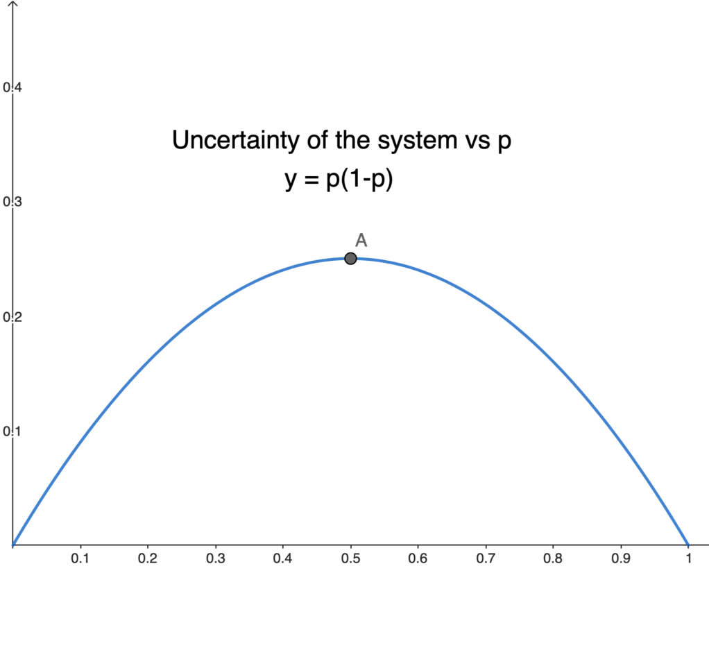
We can see that the plot increases from x=0 up until x=0.5 then it decreases.
This is what we expected, if the probabilities are equally distributed then p = 0.5 and (1-p) = 0.5 thus the uncertainty is at its peak. Also, the graph is obviously symmetric because if p = 0.2 then (1-p) = 0.8, it's the same as p = 0.8 and (1-p) = 0.2
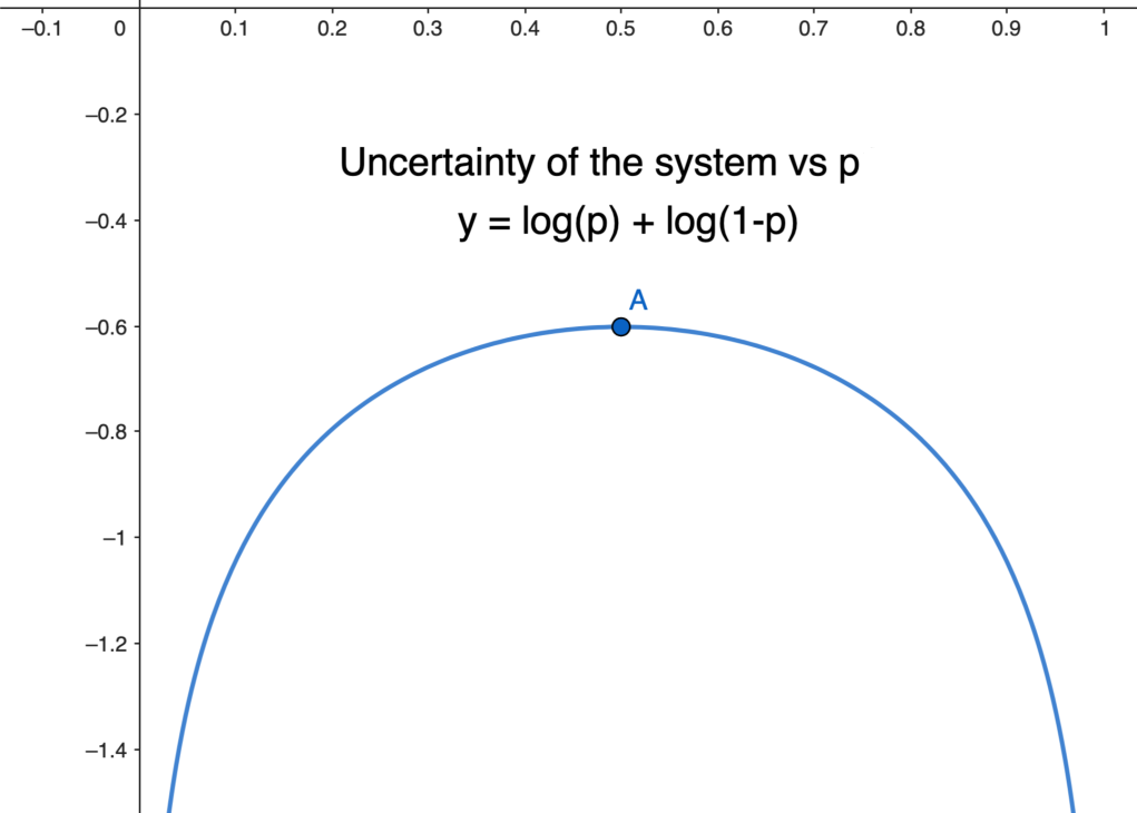
When we apply the log we get log(p(1-p)) = log(p) + log(1-p)
all the values become negatives but the relations of order are preserved, the function reaches its maximum for x=0.5 like previously. The only issue is that the functions tends to -infinity when x approaches 0 or 1.
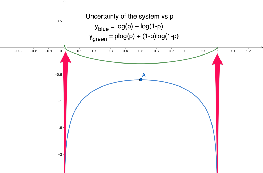
multiplying all the terms with their probabilities leads to plog(p) + (1-p)log(1-p).
As seen previously, it changes the relations of order. The reason is that it forces the function to be equal to 0 for the values x = 0 and x = 1 which flips the graph. Also, all the other values are lowered because they are being multiplied by their probability which are numbers smaller than 1.
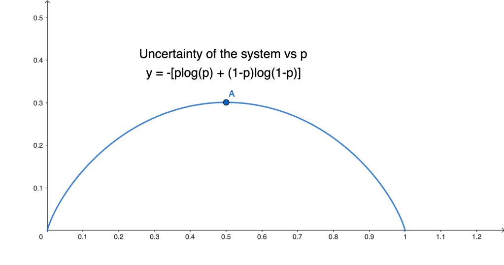
So we just multiply the whole thing by -1 to get what we want.
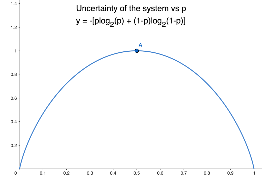
you can use whatever base you want for the log, if you choose the log base 2 then you can say that the results are in bits and the maximum value that the function can take is 1.
I still don't understand why there is a logarithmic function in the Shannon entropy formula ?
There are at least 3 good reasons :
-
It is suitable when dealing with huge or tiny numbers. For instance
$\log_{2}(100000) = 16.6$ , which makes the output much more practical. -
It coincides with Gibbs entropy) formula used in thermodynamics, and very often it is useful in science to link concepts between disciplines in order to make analogies.
-
The formula has some interesting additive properties. Feel free to read Shannon’s original paper if you are interested to know more about this topic.
How is Shanon Entropy different from variance, where is it used ?
- They both measure information but entropy is all about probabilities, that is to say you are trying to characterize a probability distribution, it doesn't care about the values themselves. This is interesting because you can compute the entropy of any categorical data which can't be done with variance. This works even if the data is non numerical, example:
["one", "one", "two", "one"] - Entropy is used in Machine Learning, especially in Decision trees as an impurity criterion.
the Decision tree splits the data at each node using impurity. The goal here is to choose the feature that minimizes the impurity. When the impurity is low it means that most of the labels are correctly predicted, in other words the uncertainty is very low. You keep adding nodes until the impurity doesn't decrease anymore. Note that this Idea goes with the previous point, the entropy trick makes the decision trees able to deal with numerical and categorical datas.
# Get probabilities associated with every label
import numpy as np
labels = [0,0,1,1,1]
values, counts = np.unique(labels, return_counts=True)
probs = counts / len(labels)
print("values:", values)
print("counts:", counts)
print("probs:", probs)

#>>> values: [0, 1]
#>>> counts: [2, 3]
#>>> probs: [0.4, 0.6]
Now, we can plug probs in the entropy method. The original formula uses the log base 2 because communication/ information was thought in terms of bits but you can choose whatever base you want.
from scipy.stats import entropy

e = entropy(probs, base=2)
print(e)
#>>> 0.9709505944546688
Finally we can define a function that takes a list of labels as input and returns its shannon entropy.
from scipy.stats import entropy

def entropy_from_labels(labels, base=2):
  """Take a list of labels as input and return its shannon entropy"""
  value, counts = np.unique(labels, return_counts=True)
  probs = counts/len(labels)
  return entropy(probs, base=base)

entropy_from_labels(labels, base=2)
#>>> 0.9709505944546688