Mutual information simply explained with example and code - A generalization of the correlation concept.
Mutual information is a very nice statistical tool that can be seen as a generalization of the correlation concept.
Indeed, the pearson's correlation allows us to find out if two variables are linearly dependent. The thing is we are not always interested only in linear relationships, that's where mutual information comes into action. It can emphasize any kind of dependance between two distributions.
Another cool thing about mutual information is that it can be used for both continuous and discrete variables.
The formula looks like this:

I've found out that many people struggle understanding what it exactly does, not because it's difficult to understand per se, but because they get confused by the notation and sometimes they also have some misconceptions. So let's dive into the subject step by step.
The core thing to understand is the concept of independence between two events A and B.
The most intuitive way to understand it is perhaps to use conditional probabilities:
Recall that P(A|B) (Probability of A given B) can be written like so:
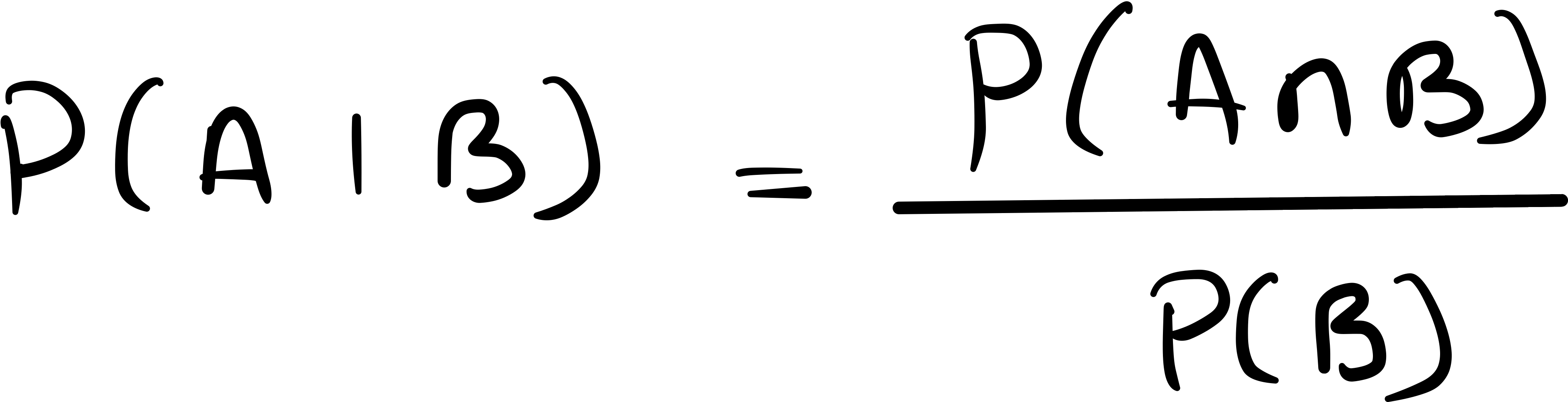
if A and B are independents it means that knowing B doesn't help you predict A, in other words, it doesn't give you any information about A.
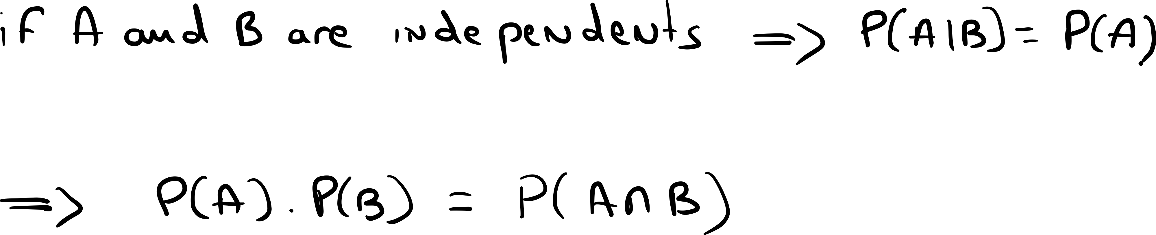
Thus the probability of A given B is simply the probability of A.
This leads to P(A and B) = P(A).P(B)
In other words, the product of the separate probabilities is equal to the probability that both events will occur.
I want to point out that most often the concept of independence is confused with the concept of mutuallly exclusive events. That is not the same thing !
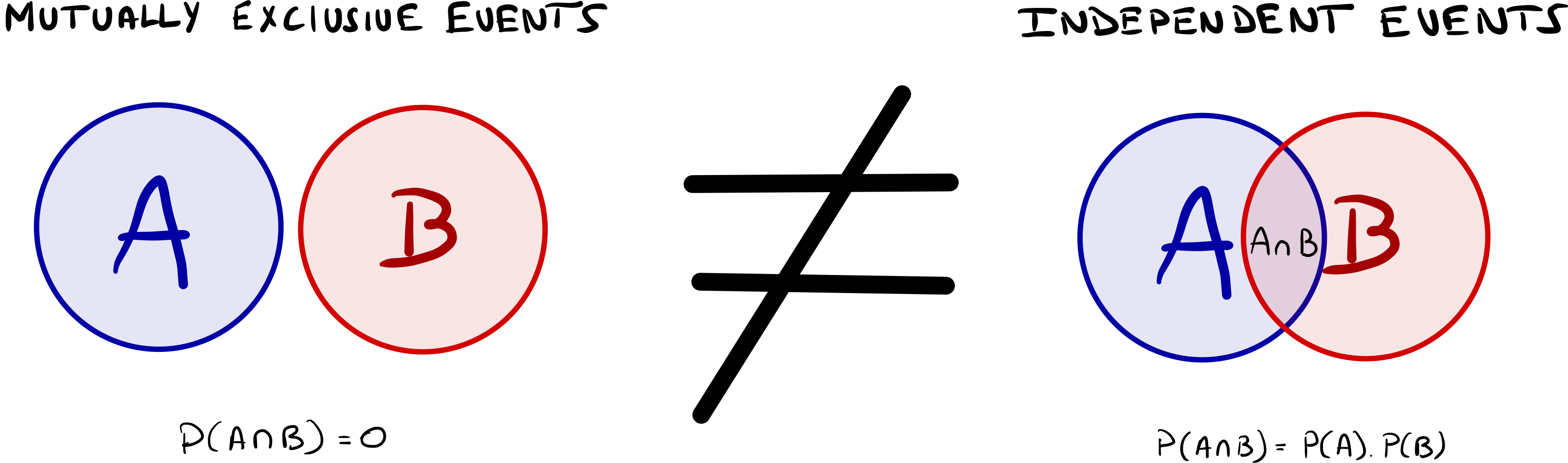
Two events are mutually exclusive if they can not occur at the same time. For instance, a tossed coin outcome can be either heads or tails, but both outcomes cannot occur simultaneously, they are mutually exclusive.
On the other hand, two independent events do occur simultaneously, simply the probability of the intersection is exactly equal to the probability that both events occur.
One last thing that might disturb you is the notation p(A,B). This is exactly the same thing as P(A and B) or P(A ∩ B).
Moreover, there is a little bit of lingo to know here:
- P(A, B) or P(A and B) or P(A ∩ B) is said to be the joint probability
- P(A) is said to be the marginal probability
- P(B) is said to be the marginal probability
- P(A | B) is said to be the conditional probability
That's it ! A probability can be either marginal, joint or conditional.
Now that you are more familiar with the key concepts, the notation and the lingo we are ready to move forward.
I've made up a dataset which features or columns are likes chocolate and gender.
There are in fact 100 lines but I won't display the whole table for obvious reasons. :D
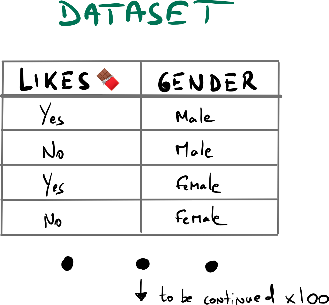
The random variable likes_chocolate has two possible events:
- Yes
- No
The random variable gender has two possible events:
- Male
- Female
From that, the idea is to see if gender affects likes_chocolate or not and vice versa.
To do so we are going to change the granularity of the study and see if the events of gender do affect the events of likes_chocolate.
A simple idea is to build up a contingency table. This is a fancy word to call a table where you count the amount of occurrences of simultaneous events. If you prefere we can also say that this is a table showing the distribution of one variable in rows and another in columns. We use this to study the correlation between the two variables. For instance the first cell which value is 23 corresponds to the number of occurrences of the simultaneous events likes_chocolate = no and gender = female.
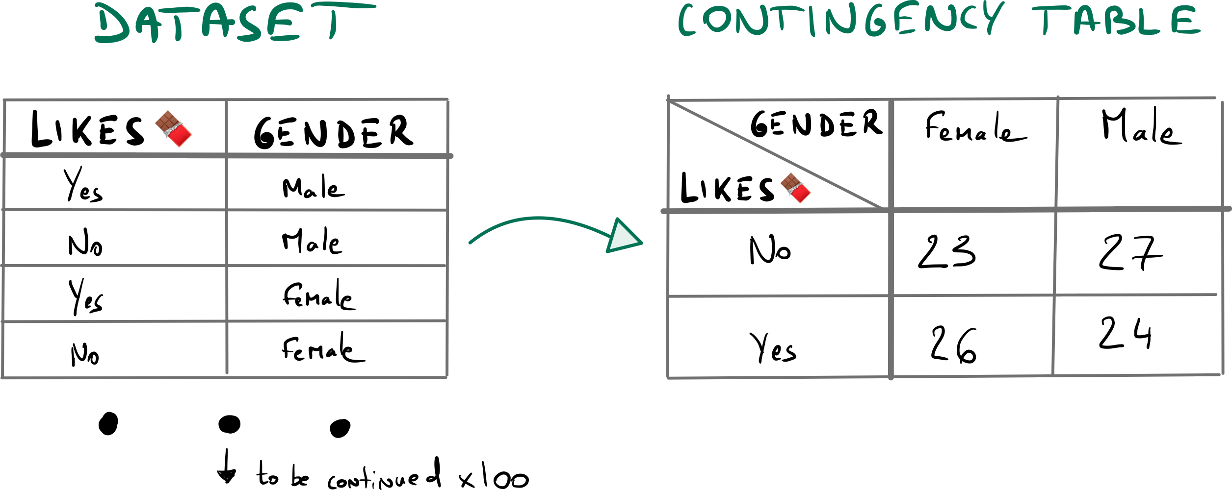
I have generated the data so that for each outcome female and male have 50% chance each to be drawn. In the same fashion, a person has 50% chance to like or not to like chocolate. In fact I've generated the data so that the variables are independent.
If the variables are perfectly independents, there is a priori no reason for a cell of the table to have more occurrences than another. We can also say that for given variables, in our case likes_chocolate and gender, if these two are independent, then there's no reason that gender affects likes_chocolate. In particular, there's no reason to observe a higher probability for the joint events gender=male and likes_chocolate = yes than for the joint events gender=female and likes_chocolate = yes. This holds true for all the other joint events (for every cell of the table).
What is interesting to understand here is that because the variables should be independent, one would expect to end end up with approximately 25 occurrences for each joint events.
That is actually what we see, although this is not exactly 25 occurences for each cell !
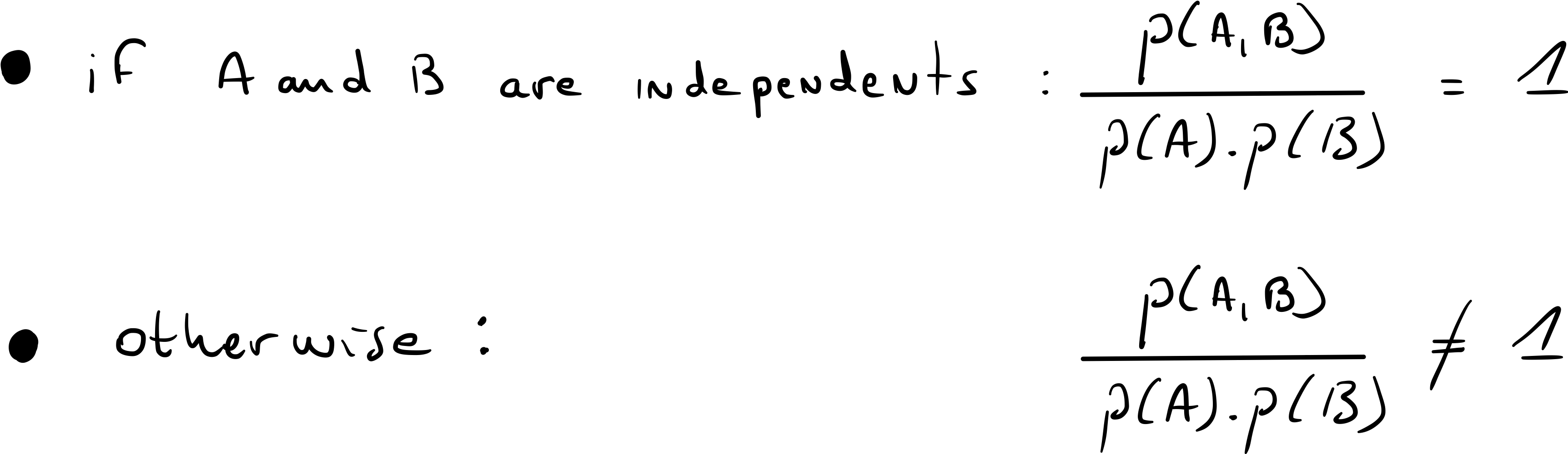
This is a toy example and frankly, we can already see that the variables are independent. However, "in the real life" everything is not perfectly balanced, so to ensure that the values of the cells remain comparable we use the following property of independence that we already spoke about:

The idea is simple. If A and B are independent then P(A and B) divided by P(A).P(B) is equal to one.
Otherwise, if the ratio is way higher or way lesser than one then there is some dependency.
So we are going to calculate how dependent are each pairs of events.
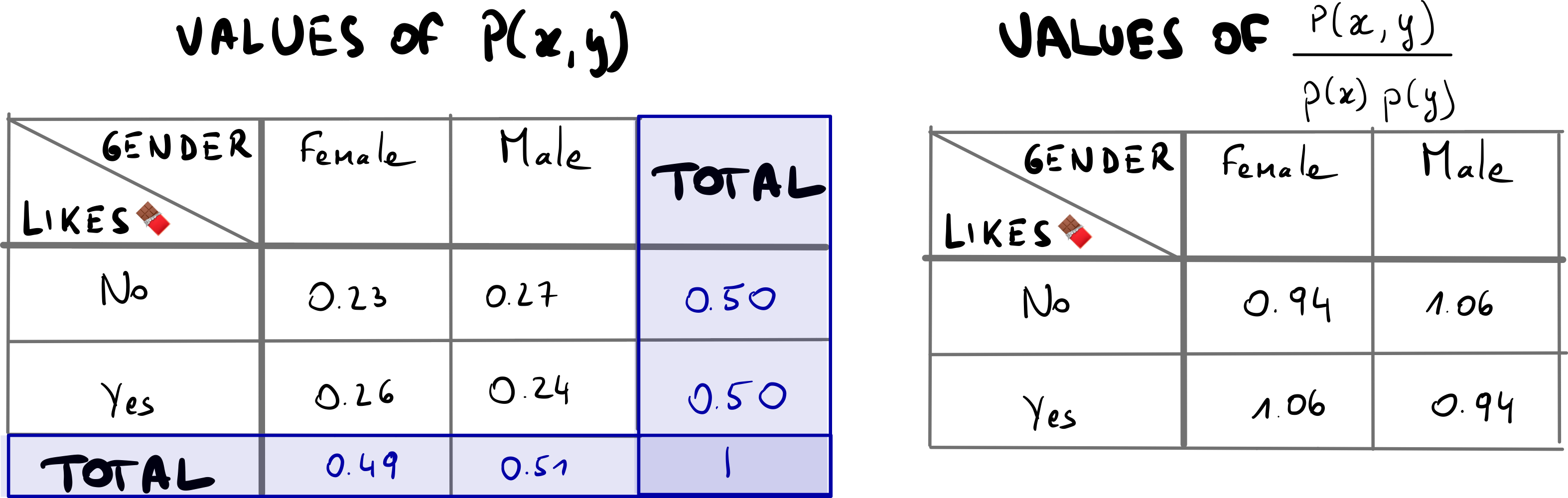
So first let's calculate all the pairs of P(A,B). The probability of A and B is simply the number of times events A and B occur simultaneously over the total number of possible outcomes (N).
here N is 100 (this is the number of lines of the dataset). As we have a contingency table, we already have the occurrences of the pairs of events, we then simply need to divide all the values by 100.
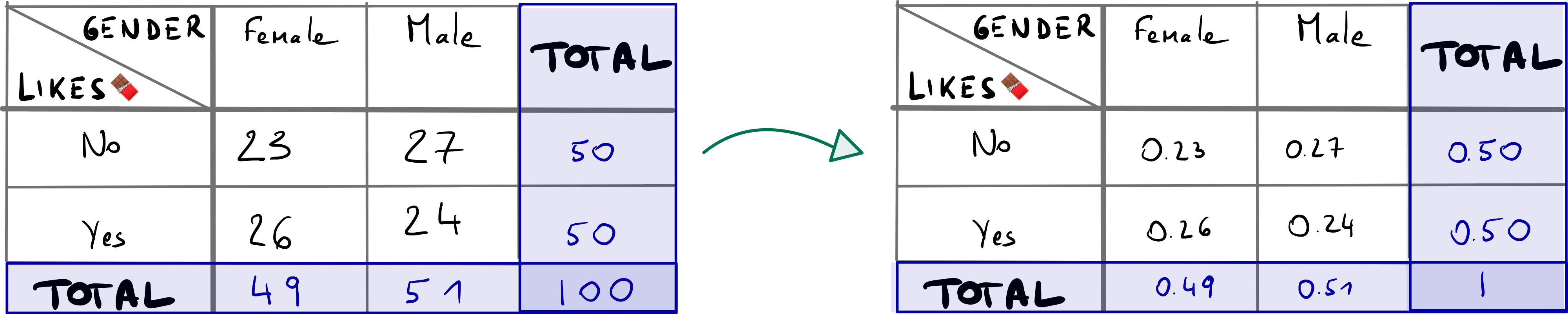
Notice that we also added a total for the lines and columns. This is helpful as we will need to calculate the marginal probabilities P(female), P(male), P(likes_chocolate) and P(dont_like_chocolate).
We can easily read for example that P(female)= 0.49.
Now the last step is to divide all the joint probabilities by the product of their marginal probabilities.
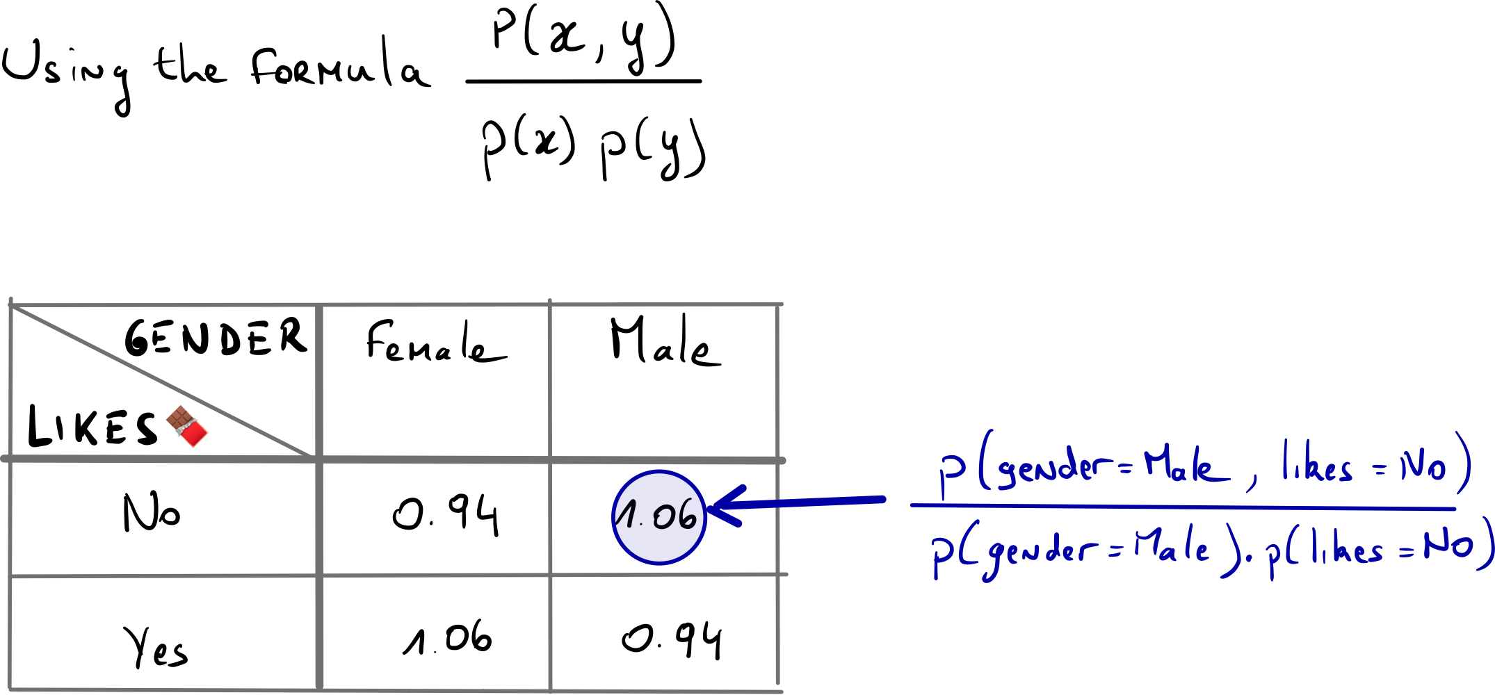
So we get a table where all the values are approximately equal to 1 meaning that all the pairs of events are independents (as expected).
Now if we were to flatten all the values of the table to make the array [0.94, 1.06, 1.06, 0.94]
and display it as a bar plot, this would look like this.
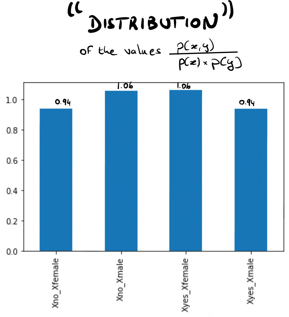
I put "distribution" in quotation marks because usually what is meant by distribution is the probability distribution which values are supposed to add up to 1. Here we just see how the values are distributed but they are not proabilities.
This is interesting to stop a moment to think of what the problem has really become.
-
If you think about that, when all the events are independents, all the values are equal to 1 so the "distribution" is flat, consequently there is no clear pattern, we can also say that events are drawn from a uniform distribution and therefore the uncertainty is maximum.
-
When the variables are very dependents, we should see some values way higher than 1 and some way lesser than 1 (because for example if a pair of events occur 80 times then there is only 20 occurrences remaining for other events) So we are favoring pairs of events over others, in other words, we are reducing uncertainty.
So this is really becoming a problem of quantifying uncertainty in the distribution. This should be somewhat reminiscent of the concept of entropy. Please read my article about entropy if you are not familiar with this concept
From there, we just calculate the entropy of the "distribution".
Entropy has this general form :

The only difference is really what's inside the log. Indeed, instead of having a probability inside, we'll have the previous quantity p(x,y)/p(x).p(y).
the log of p(x,y)/p(x).p(y) in our case has a name, it is called the pointwise mutual information or PMI.
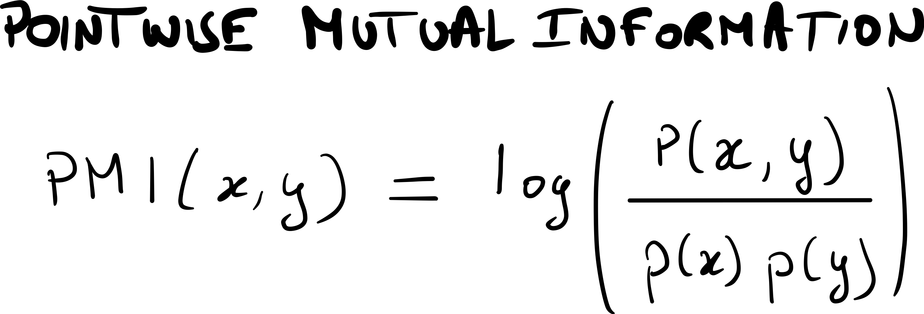
The last step is to calculate the PMI of every possible x and y weighted by the probability p(x,y) that x and y occur together. This weighted average measures how much we expect the variables to be dependent of each other. We can also say that this measures how much we expect the variables to predict each other.
This leads us to the formula.

Or we can also write this in a more explicit way
Applied to our example, and with the help of our previous tables the calculation is as follows:
I(X, Y) = 0.23*log(0.94) + 0.27*log(1.06) + 0.26*log(1.06) + 0.24*log(0.94)
I(X, Y) ≈ 0
-
The mutual information is almost equal to 0 which means that the variables X=
likes_chocolateand Y=genderdon't share any information together, that is they are independent. -
A usueful property to know is that the mutual information can never be lesser than 0.
-
When the mutual information is greater than 0 we can say that there is some dependency. The more the value is high the more there is dependency between variables. Unlike pearson's correlation, the upper bound of the mutual information is not 1. In fact there is an upper bound but it depends on your data. Usually it doesn't matter to know the upper bound as you just need a relative value so that you can sort all the features X_i that are the most correlated with a feature Y for instance. By the way, I'll show you how you could use mutual information as a feature selector in a bit :)
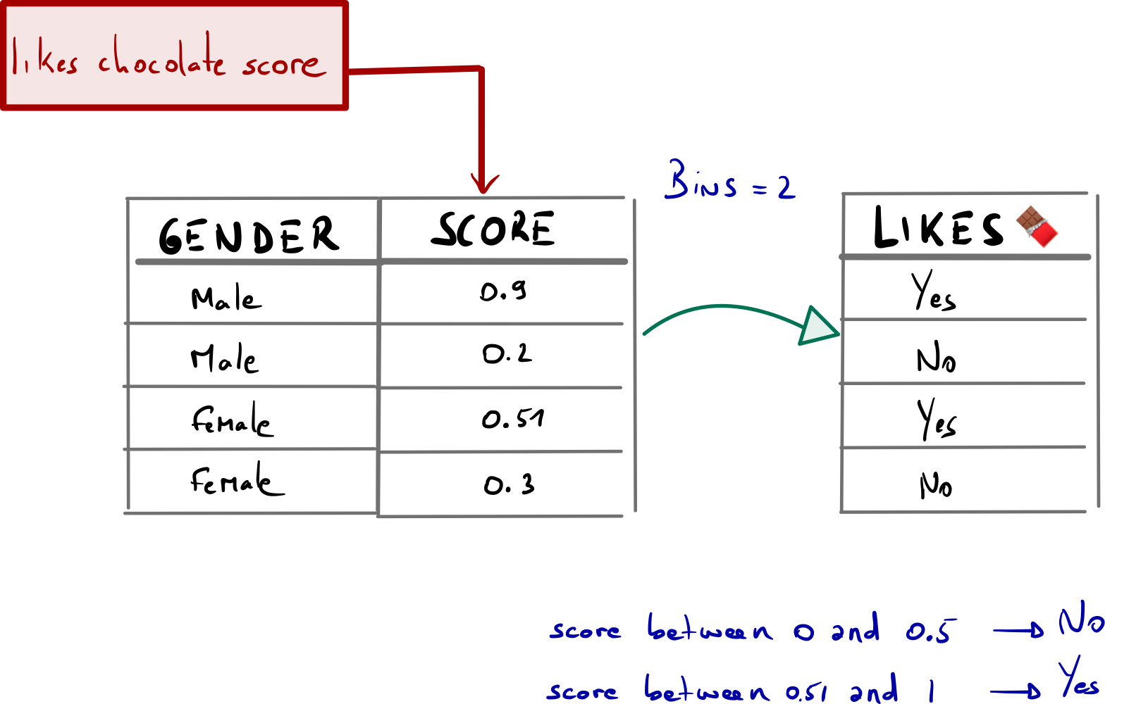
Normally we can only use categorical variables with mutual information. The trick here is to transform continuous variables into categorial variables.
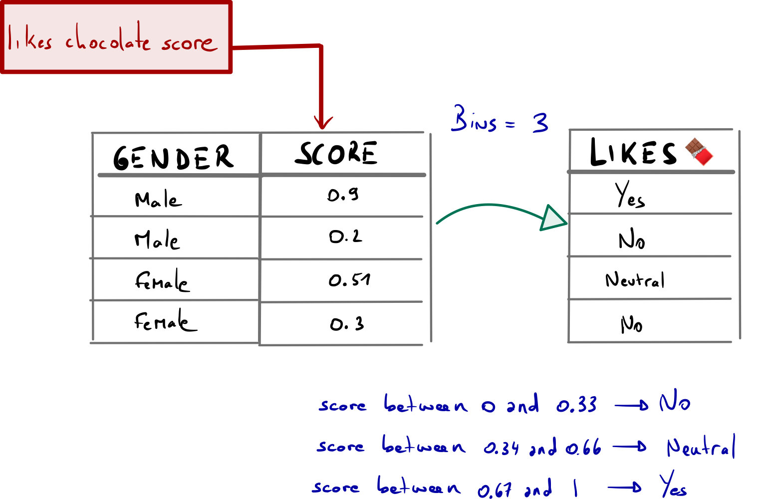
One way to do this is to use binning, which involves dividing the range of values of a continuous variable into a set of bins or intervals and assigning each observation to its corresponding bin.
Here a simple example with bins=2 and bins=3. The number of bins is the number of categories you want to build up. In the example, we have a continuous variable lkes_chocolate_score that we are going to discretize or to transform into categories.
You can use the following code to test de dependency of several features of X against the target variable Y
from sklearn.feature_selection import mutual_info_classif
# Load the iris dataset
iris = load_iris()
# Separate the features (X) from the target (y)
X = iris.data
y = iris.target
# Compute the mutual information between each feature and the target
mutual_info = mutual_info_classif(X, y)
# Print the mutual information scores for each feature
for i in range(len(mutual_info)):
print(f"{iris.feature_names[i]}: {mutual_info[i]:.3f}")[/code]
sepal length (cm): 0.488
sepal width (cm): 0.258
petal length (cm): 0.985
petal width (cm): 0.969
In this example, we first load the iris dataset from the sklearn.datasets module. We then separate the features (X) from the target (y).
Next, we use the mutual_info_classif function to compute the mutual information between each feature and the target. It returns an array of mutual information scores, one for each feature.
Finally, we print out the mutual information score for each feature using a loop. The output will show the mutual information score for each of the four features in the iris dataset.
To select features based on mutual information, we have to choose the features with the highest scores. These features are considered to have the strongest relationship with the target variable and are likely to provide the most valuable information for predicting the target. In our example petal_width and petal_length appear to be the features that are highly related to the target variable.
That's it for today, thank you for reading !